TLDR: my home emitted 1423.83 kg CO₂ in 2024, down from 2000.94 in 2022. Read the full manuscript including R code here
For a recent project I’m working on modeling carbon emissions, which got me interested in the carbon emissions caused by my home. Luckily, I have been measuring my utilities consumption for some time, and thus can quite accurately calculate my home’s emissions.
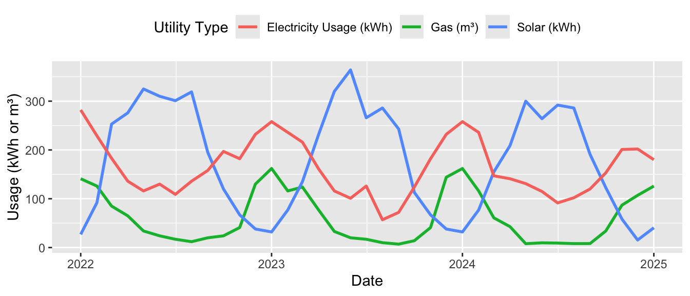
Utilities consumption
assuming the following consumption pattern:
 Load utility data
data_utilities <- read.csv("data/utilities.csv", sep=";", dec=",")

# Date format handling
data_utilities$date <- as.Date(paste0("01-", data_utilities$date), format = "%d-%m-%Y")

# Plot
library(ggplot2)

ggplot(data_utilities, aes(x = date)) +
  geom_line(aes(y = Gas, color = "Gas (m³)"), linewidth = 1) +
  geom_line(aes(y = Solar, color = "Solar (kWh)"), linewidth = 1) +
  geom_line(aes(y = Energy, color = "Electricity Usage (kWh)"), linewidth = 1) +
  labs(x = "Date",
       y = "Usage (kWh or m³)",
       color = "Utility Type") +
  theme(
    legend.position = "top",
    legend.justification = "center"
  )
Emissions of energy production
To quantify and compare the warming effects of different kind of emissions, the IPPC proposes using the Global Warming Potential (GWP), which can be used to express the warming effect of different emissions to that of CO₂. To calculate our total emissions, we must first determine the emissions caused by the energy production.
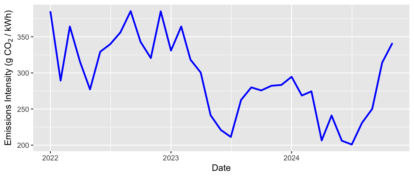
Electricity
The emissions of electricity production depends on the source of the energy, which changes minute-by-minute. During day, a lot of green solar power is generated, and during peaks, gas turbines kick in. Exact information on the current national energy mix is publicly available. Ember-energy calculates the CO₂ emissions based on the energy mix, and has an API (email required) which provides the following numbers:
See also: CBS emissie rendementen elektriciteit
# Energy Intensity data
# ember-energy requires an API key. This script will look for the existence of energy_intensity.csv, and otherwise requires an API key to fetch new data.
API_KEY <- "YOUR-API-KEY"

# Check if the file 'energy_data.csv' exists
if (file.exists("data/energy_intensity.csv")) {
  # print("File 'energy_intensity.csv' already exists.")
  data_energy_intensity <- read.csv("data/energy_intensity.csv")
} else if (API_KEY == "YOUR-API-KEY") {
  print("No valid ember-energy API key")
} else {
  # Requesting the energy intensity data
  # Define the URL and the parameters
  url <- "https://api.ember-energy.org/v1/carbon-intensity/monthly"
  params <- list(
    entity = "Netherlands",
    start_date = "2022-01",
    include_all_dates_value_range = "false",
    api_key = API_KEY
  )
  library(httr)
  library(jsonlite)

  # Send the GET request
  response <- GET(url, query = params, add_headers("accept" = "application/json"))

  # Convert teh response to JSON
  data <- content(response, as = "text")
  data_json <- fromJSON(data)

  # Check if the JSON contains data or an error
  if (length(data_json$data) == 0) {
    print("Something went wrong with the API request: No data found in 'data_json$data'.")
  } else {
    energy <- as.data.frame(data_json$data)
    data_energy_intensity <- data.frame(
      date = energy$date,
      emissions_intensity_gco2_per_kwh = energy$emissions_intensity_gco2_per_kwh
    )

    # As energy_intensity.csv does not exist, we save the data
    write.csv(data_energy_intensity, "data/energy_intensity.csv")
  }
}


# Ensure 'date' is in Date format
data_energy_intensity$date <- as.Date(data_energy_intensity$date)


# Plot
ggplot(data_energy_intensity, aes(x = date, y = emissions_intensity_gco2_per_kwh)) +
  geom_line(color = "blue", linewidth = 1) +
  labs(
    x = "Date",
    y = expression("Emissions Intensity (g CO"[2] ~ "/ kWh)")
  )
To calculate the emissions caused by our energy consumption, we should account for the differing CO₂ emissions as follows:
$$
\text{CO}_2 = \sum_{i=1}^{n} E_i \times F_i
$$
With \( \text{CO}_2 \) as the total produced CO₂ in grams, \( E_i \) the electricity usage for month \( i \) in kWh, and \( F_i \) the emissions intensity in \( \text{g CO}_2/\text{kWh} \).
Gas
Calculating the exact emissions caused by gas production is somewhat more complex as gas distributors measure the gas-usage as volume (m³) which is dependent on the temperature, pressure and gas mix, all of which are subject to change. Gas distributors solve this by multiply the measured volume with a correction value to determine the caloric value of the consumed gas (also see wobbe index). These corrections can be found on the final invoice.
The Netherlands Enterprise Agency (RVO) has calculated the emission factor for natural gas to be 56.34 kg CO₂ per GJ of energy. This only includes the emissions caused by burning the gas, not from producing it. The exact number differs by ±2% per year due to differences in the national gas mix, for instance through higher LNG imports.
The CBS reports that 1 GJ of natural gas corresponds to 31.6 m³, thus we can calculate the emissions per m³ as follows:
$$
\text{CO}_2 = \sum_{i=1}^{n} E_i \times F_i
$$
Since:
$$
1 \text{ GJ} = 31.6 \text{ m}^3
$$
we can compute:
$$
\frac{56.34}{31.6} \text{ kg/m}^3
$$
which simplifies to:
$$
1.78 \text{ kg CO}_2 \text{ per m}^3
$$
As the deviations for the emissions of the gas mix are ~2%, we simplify the calculation by not accounting for them.
Calculations
From the emission factors per energy type the final formula can be determined:
$$
\text{CO}_2 = \left( \sum_{i=1}^{n} E_i \times F_i \right) + \left( G \times 1,78 \right)
$$
With $\text{CO}_2$ as the total produced CO₂ in grams, $E_i$ the electricity usage for month $i$ in kWh, $F_i$ the emissions intensity in $kg CO₂/kWh$ for that specific month $i$. $G$ the total gas usage in m³ Plugging our usage data into this formula gives us the following emissions:
# Merge datasets by date
data_emissions <- data_utilities %>%
  inner_join(data_energy_intensity, by = "date") %>%
  mutate(
    Electricity = (Energy * emissions_intensity_gco2_per_kwh) / 1000,  # Convert g to kg
    Gas = Gas * 1.78  # kg CO2 per m³) %>%
  select(date, Electricity, Gas)  # Keep relevant columns

# Convert to long format for ggplot
data_emissions_long <- data_emissions %>%
  pivot_longer(cols = c(Electricity, Gas),
               names_to = "Source", values_to = "Emissions")

if (knitr::is_html_output()) {
  # Interactive Stacked Area Plot
ggplot(data_emissions_long, aes(x = date, y = Emissions, fill = Source)) +
  geom_area(alpha = 0.6) +  # Stacked area plot
  labs(
    x = "Date",
    y = expression("CO"[2] ~ " Emissions (kg)"),  # Fix CO₂ subscript
    fill = "Emission Source"
  ) +
  theme(
    legend.position = "top",  # Place legend at the top
    legend.justification = "center"  # Center-align the legend
  )
} else {
  # Static Stacked Area Plot (ggplot2)
  ggplot(data_emissions_long, aes(x = date, y = Emissions, fill = Source)) +
    geom_area(alpha = 0.6, position = "stack") +  # Stacked area plot
    labs(
      x = "Date",
      y = expression("CO"[2] ~ " Emissions (kg)"),  # Fix CO₂
      fill = "Emission Source"
    ) +
    theme(
      legend.position = "top",
      legend.justification = "center"
    )
}

# For the tables:
data_emissions$total <- data_emissions$Gas + data_emissions$Electricity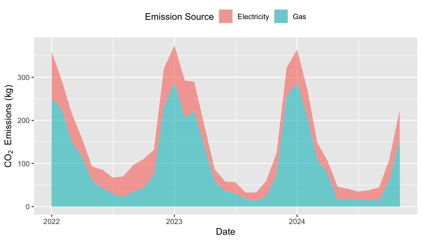
note: emissions on monthly basis
library(dplyr)
library(knitr)

# Ensure 'date' is in Date format
data_emissions$date <- as.Date(data_emissions$date)

# Extract year from date
data_emissions$year <- format(data_emissions$date, "%Y")

# Aggregate emissions per year
yearly_emissions <- data_emissions %>%
  group_by(year) %>%
  summarise(
    `Gas emissions (kg CO₂)` = sum(Gas, na.rm = TRUE),
    `Electricity emissions (kg CO₂)` = sum(Electricity, na.rm = TRUE),
    `Total emissions (kg CO₂)` = sum(total, na.rm = TRUE))

# Display the table in Quarto
kable(yearly_emissions, format = "html", digits = 2, align = "c")| Year | Gas emissions (kg CO₂) | Electricity emissions (kg CO₂) | Total emissions (kg CO₂) |
|---|---|---|---|
| 2022 | 1279.82 | 721.12 | 2000.94 |
| 2023 | 1361.70 | 551.89 | 1913.59 |
| 2024 | 970.99 | 452.84 | 1423.83 |